
A brief introduction to the Generic Mapping Tools (GMT 5.1.x)
GMT operates on a UNIX style command line interface. If you don’t know what that means, that’s fine, I’m going to break it down for you here. Basically, it means that GMT operates by you typing a string of characters that tell the system what program to run and how exactly to run that program. So, the first thing in any command is the call to the GMT suite within your system, followed by the name of the GMT program you wish to run. This is followed by a series of switches that give the GMT program specific instructions on what to do. Each switch has a series of arguments associated with it that further detail to the program how exactly you want the program executed. Let’s take a look at the following command:
gmt pscoast -R-87/-69/31/45 -JM10c -Xc -Yc -B2 -Dl -A0/0/2 -Ggrey -W > map.ps
Wow! Looks complicated, huh? Well let’s break it down and work through it.
The first part is gmt pscoast; this is the name of the program we are calling (it is a program for accessing and plotting shoreline, territory border, and other datasets) The next part is -R-87/-69/31/45. There are several GMT switches that exist as options in many GMT programs (e.g. -R,-J,-G) as the same switch, however this is not always the case. In this instance, the switch (-R is followed by the argument (-87/-69/31/45), in this case the boundaries of the area you want to plot in the order left/right/bottom/top, in decimal degrees.
Next we see -JM10c. Okay, this is a set of one switch, and two arguments for that switch. The -J tells pscoast that the following text input is about what map projection to use when plotting the data. The M indicates to use the Mercator Projection type, and lastly the 11c indicates that the entire plot should have the longest axis measure 11 centimeters. The -Xc and -Yc switches and arguments tell the program to (c)enter the plot in the output page.
The next part, -B2 tells the pscoast program how to draw the border of the map plot. The switch is -B, and the arguments indicate to break the border every 2 decimal degrees with a mark.
-D is the switch for selecting the level resolution to use in plotting the datasets. Five levels exist: (f)ull, (h)igh, (i)ntermediate, (l)ow, and (c)rude. We will use the low resolution, because we are plotting a large area.
The -A switch indicates what level of coastlines to plot. Without going into too much detail, explained here, the selection we made tells the program to plot the coastline and all lakes.
The next switch, -G is a tricky one, because depending on the program you are using has different meanings. In this program it means the color fill of land (or “dry”) areas; we have selected grey. The other common meaning for this switch is to specify an output file, however this can be ignored for the moment. Also, we will not do so here, but another popularly included switch is to use -S to specify the fill color for “wet” areas.
-W specifies to trace the shorelines. Typically there are “pen-specifying” arguments to follow the switch, but the default will be fine for our purposes now.
Now the last part, > map.ps, simply tells pscoast where to write the output file. The name is chosen by you, but needs the file extension “.ps”.
Now look back at the command we gave, that long string of seemingly arbitrary characters should seem pretty simple now, each character with a special and important meaning.
The command we dissected produces the output below. It sure is not beautiful yet, but we can see that the command worked.
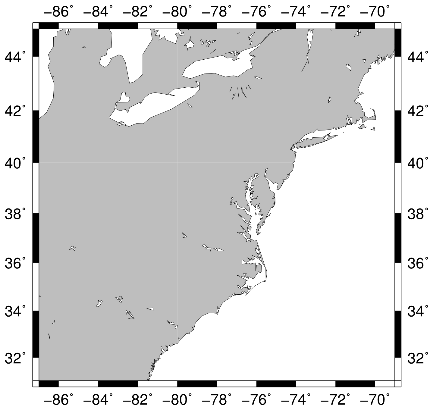
Maybe you have noticed this is a map of a section of the East Coast of the United States of America. As an America, I’ll probably draw a lot of the content I post from this area, but I promise I’ll try to keep it interesting.
Note that we have just scratched the surface of the options that the pscoast program has, but this should give you a good idea of the basic syntactical nature of GMT program commands. In the next chapter of this series, we’ll make a slightly more complicated map and continue building our Generic Mapping Tools skill set!
Click here for the next tutorial: “Writing scripts to build maps with the Generic Mapping Tools (GMT 5.1.x)”.