Adding real data into GMT map, making a hillshade, and positioning

Alright, let’s get down to business plotting some real data on a map. Grab the zip file here, and uncompress it in the folder you want to build a map in. The zip contains the data to map, as well as  on of my favorite color palettes from cptcity by M. Burak Yilkilmaz (file named mby.cpt).

Here’s the end product of this tutorial, we’re going to make two maps, the first will be a simple data map, and the second a hillshaded version of the same map. We’ll also learn how to position them side by side like below.

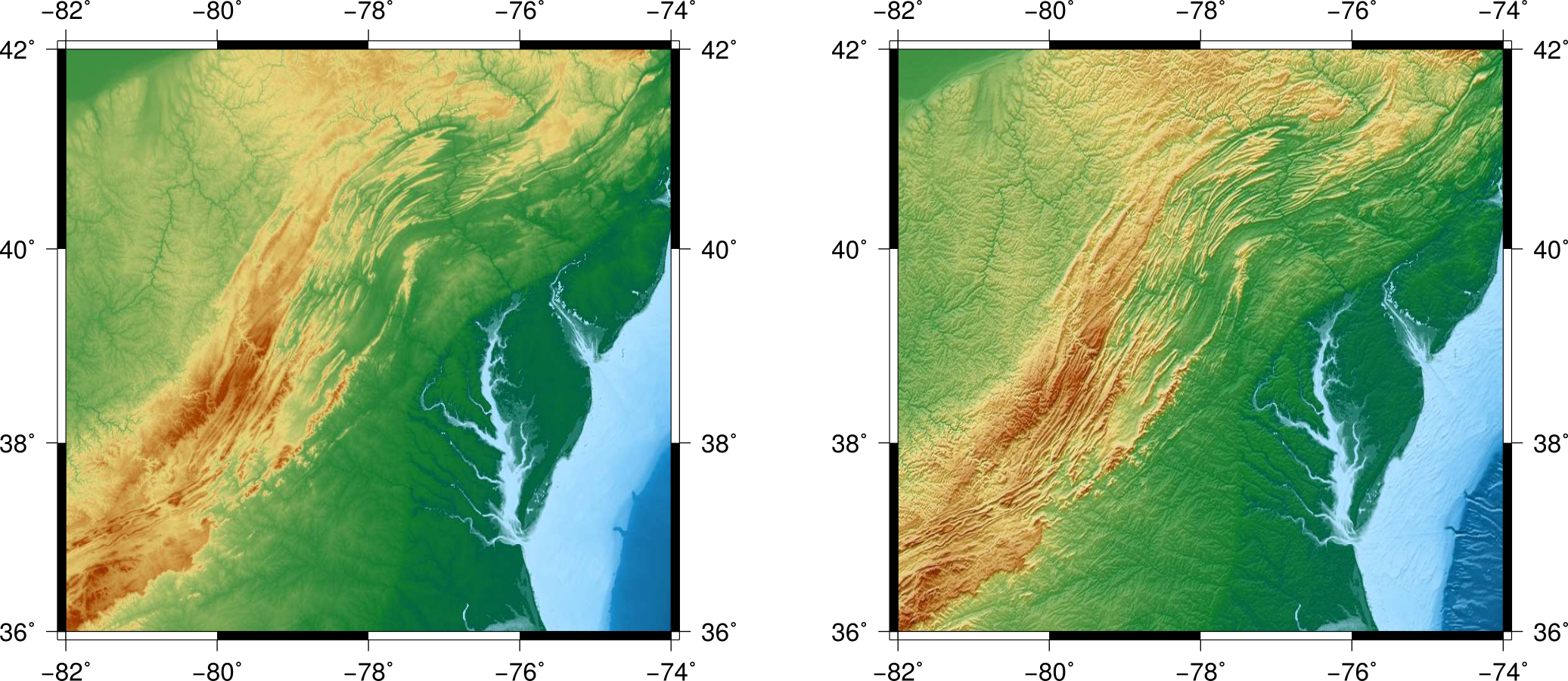
We’ll start by plotting a simple map, with just the data represented as different colors (left side of the map). The data we’re plotting are from a digital elevation model (DEM), and of Eastern North America. Making this image is simple, we simply need to call

gmt grdimage real_data.nc -R278/286/36/42 -JM4 -B2WESN -Xc -Yc -Cmby.cpt -V > flat.ps

where you already know most of the switches above. grdimage is a GMT tool that you can use to plot any data stored in the netCDF format. To color the image based on the values in the .nc file, we need to use a color palette. The color palette is called with the -C switch, followed by the name of the color palette. More on color palettes in a future tutorial though.

Now, let’s talk about hillshades. A hillshade (also known as shaded relief) is an element of a map that adds depth to topography. It is essentially simulating a light source and the shadows cast on the landscape from the hills onto the valleys. Making one in GMT is straightforward but requires a few steps. The main step of the process is done first with grdgradient. We use the following command

gmt grdgradient real_data.nc -Ghillshade-grad.nc -A345 -Ne0.6 -V

In this command, -G has a different meaning than in this tutorial; another common use of the -G switch is to give the name of the output file for the command. -A is the azimuth from which the light source should be directed, and -Ne is a normalization parameter for the output from the calculation, just use 0.6.

Then, we will ensure that the shaded relief map is reasonably balanced by normalizing it again along a Gaussian distribution

gmt grdhisteq hillshade-grad.nc -Ghillshade-hist.nc -N -V

Finally, in order to ensure the values are between -1 and 1, a final step required for creating the intensity file needed for a hillshade to the image. We do this by dividing by some value just larger than the range of values in the histogram equalized grid file. Let’s find this range by looking at the info for this file.

gmt grdinfo hillshade-hist.nc
	hillshade-hist.nc: Title: Produced by grdhisteq
	hillshade-hist.nc: Command: grdhisteq hillshade-grad.nc -Ghillshade-hist.nc -N -V
	hillshade-hist.nc: Remark: Normalized directional derivative(s)
	hillshade-hist.nc: Gridline node registration used [Geographic grid]
	hillshade-hist.nc: Grid file format: nf = GMT netCDF format (32-bit float), COARDS, CF-1.5
	hillshade-hist.nc: x_min: 278.004166667 x_max: 286.004166667 x_inc: 0.00833333333333 name: longitude [degrees_east] nx: 961
	hillshade-hist.nc: y_min: 35.9958333333 y_max: 41.9958333333 y_inc: 0.00833333333333 name: latitude [degrees_north] ny: 721
	hillshade-hist.nc: z_min: -4.67873573303 z_max: 4.67873573303 name: Elevation relative to sea level [m]
	hillshade-hist.nc: scale_factor: 1 add_offset: 0
	hillshade-hist.nc: format: netCDF-4 chunk_size: 138,145 shuffle: on deflation_level: 3`

So we will use 5 as our divisor, in the command

gmt grdmath hillshade-hist.nc 5 DIV = hillshade-int.nc

which takes our -hist file and divides every grid cell by 5, putting it within the range of -1 to 1.

Finally, we use

gmt grdimage real_data.nc -R278/286/36/42 -JM4 -B2WESN -Xc -Yc -Ihillshade-int.nc -Cmby.cpt -V > shaded.ps

the grdimage tool again, in almost exactly the same way as before, except adding the -I switch with our normalized intensity file as the input.

Now, to put the two images side by side, we need to set different -X and -Y targets for each image. These switches set the offset of the lower-left corner of the PostScript layer being produced, from the last reference point used on the PostScript page. The a argument can be added to the switches to reset the reference point to the lower-left corner of the page. Try using -Xa1 -Yc for the flat image and then overlay the hillshade image at -Xa6.5 -Yc. Remember, you’ll need to add in -K, -O, and >> in order to produce a multi-layer map.

See if you can make it work by yourself, but if you need a hint, you can get the script I used from here.