Building a simple delta numerical model: Part II

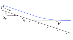
Taking the simpler form of the backwater equation, that is, assuming that width does not vary over the channel reach, we find an expression for changing flow depth \(H\) along the channel streamwise coordinate \(x\) (Equation 1):

\[\frac{dH}{dx} = \frac{S-C_f \textrm{Fr}^2}{(1-\textrm{Fr}^2)}\]

where \(S\) is the channel bed slope, \(C_f\) is the dimensionless coefficient of friction, and \(\mathrm{Fr}\) is the Froude number (Equation 2):

\[\mathrm{Fr}^2 = \frac{ {q_w} ^2}{gH^3}\]

A couple quick notes about the overall delta model we are developing herein:

1. The code for this entire model will be developed in Matlab syntax, however, the math is all just math, and the code could easily be translated to another programming language.
2. The model will be set up for the conditions of the Mississippi River, to what I feel are the best constraints published in the literature. Surely not everyone will agree with some of my choices.

We set up our model domain by defining some parameters:

L = 1200e3; % length of domain (m)
nx = 400; % number of nodes (+1)
dx = L/nx; % length of each cell (m)
x = 0:dx:L; % define x-coordinates
start = 63; % pin-point to start eta from (m)
S0 = 7e-5; % bed slope
eta = linspace(start, start - S0*(nx*dx), nx+1); % channel bed values
H0 = 0; % fixed base level (m)
Cf = 0.0047; % friction coeff

Each of these terms are necessary for defining the boundary conditions the backwater calculation requires. We will additionally need to define the water discharge (\(Q_w\)), and it’s width averaged derivative \(q_w = Q_w / B\), where \(B\) is the channel width. We’ll use a fixed width of 1100 m (Nittrouer et al., 2012) and a discharge of 10,000 m³/s; since width is fixed in our model, \(q_w = 31.8182 \) m²/s.

Finally, to solve the above backwater equation, we’ll need to find the local slope at all nodes—our bed holds a constant slope so we could just skip this step and send \(S_0\) directly into the calculation, but we’ll be wise beyond our present experience, and prepare our calculation now for the future when our bed slope is constantly changing in time and space. A simple slope calculation is completed by a central difference calculation, applying forward difference and backward difference calculations at the domain upstream and downstream boundaries, respectively.

function [S] = get_slope(eta, nx, dx)
  % return slope of input bed (eta)
  S = zeros(1,nx+1);
  S(1) = (eta(1) - eta(2)) / dx;
  S(2:nx) = (eta(1:nx-1) - eta(3:nx+1)) ./ (2*dx);
  S(nx+1) = (eta(nx) - eta(nx+1)) / dx;
end

As described in the previous section, we will use a predictor-corrector scheme to find a solution to Equation 1. This is not meant to be a comprehensive guide on solving ODEs, and so I will only summarize the method here.

1. We first can evaluate the flow depth \(H\) at the downstream boundary, where elevation is fixed (\(H = H_0 - \eta = 21\) m).
2. Then we predict the value at the next upstream node by solving Equation 1 for \(dH/dx\) at our known downstream-most node, using the inputs described above and \(H\) and \(S\) at the known node. This yields \(dH/dx|_p = 6.5784e^{-05}\).
3. Multiplying \(dH/dx|_p\) by \(dx = 3000\) m and subtracting this change from the known \(H\) at the downstream-most node, we find our predicted value \(H_p\) for the next upstream node.
4. We now repeat the evaluation of Equation 1 with the same inputs except using our new \(H_p\) value in Equation 2. This yields our corrected change in flow depth over \(x\): \(dH/dx|_c = 6.5663e^{-05}\).
5. We then combine the results of these two predictions in flow depth change to give our best solution to the ODE Equation 1 at the downstream node. We combine the values using the trapezoidal rule for \(H_i\) = \(H(i+1) - ((0.5) \times (dH/dx|_p + dH/dx|_c) \times dx)\), giving a predicted change in flow depth of \(0.1972\) m, for a depth at \(H_i\) of \(20.8028\) m (it was \(21\) m at the downstream node).
6. repeat steps 2–5 solving for each node moving up the model domain until the final node is determined.

This method is fairly stable for most discharges, but may fail when discharge is very low. In thsi case, the backwater region becomes condensed, and the rate of change in \(H\) becomes very large over a very small distance. My code for the predictor corrector implementation can be found as the get_backwater_fixed() function within the complete backwater_fixed model. Below is a video showing the results of a range of input discharges to our model.

and a still multi-surface example to demonstrate the variability.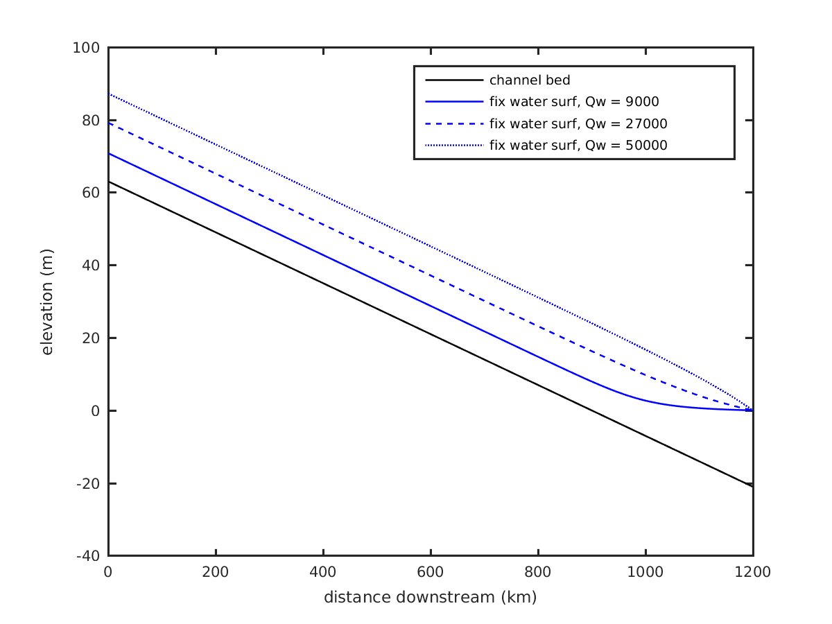

The low and moderate discharge water surface curves in the above figure (solid and dashed lines) demonstrate the classical convex-up (aka M1, e.g., Chow, 1959) condition that characterizes lowland delta systems during most of the time. The third, high discharge, water surface profile exemplifies a convex-down water surface profile. This condition, called the M2 condition has been recently demonstrated to have importance to the cyclic processes of avulsion and delta-lobe growth (e.g., Chatanantavet et al, 2012; Ganti et al., 2016).

References

1. Nittrouer et al., Spatial and temporal trends for water-flow velocity and bed-material sediment transport in the lower Mississippi River. 2012. Geological Society of America Bulletin (Table 1).
2. Chow, Ven Te. Open Channel Hydaulics. N.p., 1959. Print. McGraw-Hill Civil Engineering Series.
3. Chatanantavet, Phairot, Michael P. Lamb, and Jeffrey A. Nittrouer. Backwater Controls of Avulsion Location on Deltas. 2012. Geophysical Research Letters 39.1
4. Ganti, V., A. J. Chadwick, H. J. Hassenruck-Gudipati, B. M. Fuller, and M. P. Lamb. Experimental River Delta Size Set by Multiple Floods and Backwater Hydrodynamics. 2016. Science Advances 2 (5).

This material is based upon work supported by the National Science Foundation (NSF) Graduate Research Fellowship under Grant No. 145068 and NSF EAR-1427177. Any opinion, findings, and conclusions or recommendations expressed in this material are those of the author(s) and do not necessarily reflect the views of the National Science Foundation.