
Building a simple delta numerical model: Part III
In this part of “Building a simple delta numerical model”, we’ll simply develop a module for calculating sediment transport at all locations within our model domain. This is naturally a critical piece of the model to get right, because the magnitude of sediment transport that occurs within the delta system will have a direct correlation with the magnitude of geomorphic change to the delta system. Just as before, we’ll be working our module for the Mississippi River, and so we will use the Engelund and Hansen, 1967 formulation for bed-material load sediment transport.
It is worth noting here that there are countless sediment transport equations published within the literature, with applicability for different scenarios, covering the entire range of alluvial rivers, the shelf environment, to turbidity currents. A nice review of some relations is given by Garcia, 2008, who produces the plot below with six selected relations, where \(\tau^*\) is shear stress (Shields number) and \(q^*\) is a dimensionless sediment transport.
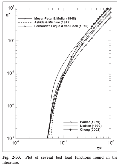
The only points I hope to make with this figure are that stress and transport are nonlinearly related, and that many of the relations are quite similar. In fact, the majority of sediment transport equations are based on an excess-shear stress formulation, where, as shown above, the sediment transport prediction scales with the shear stress. The Engelund and Hansen, 1967 equation is given in its dimensional form by (Equation 1)
\[q_s = \beta \sqrt{RgD}D\frac{0.05}{C_f}\left(\frac{\tau}{\rho RgD}\right)^{2.5}\]where \(q_s\) is the sediment transport per unit width (m2/s), \(\beta\) is an adjustment coefficient discussed below, \(R=1.65\) is submerged specific gravity of the bed sediment, \(g = 9.81\) m/s2 is gravitational acceleration, \(D\) is the grain size in question, \(C_f\) is the coefficient of friction, \(\rho= 1000\) kg/m3 is the fluid density, and \( \tau = \rho C_f U^2 \) is the fluid shear stress, where \(U\) is depth-averaged fluid velocity.
The solution to this equation is obtained by simple algebra, and so I will display the code calculations below without any explanation.
U = Qw ./ (H .* B0); % velocity
function [qs] = get_transport(U, Cf, d50, Beta)
	% return sediment transport at capacity per unit width
	% 1000 = rho = fluid density
	% 1.65 = R = submerged specific gravity
	% 9.81 = g = gravitation acceleration
	u_a = sqrt(Cf .* (U.^2));
	tau = 1000 .* (u_a.^2);
	qs = Beta .* sqrt(1.65 * 9.81 * d50) * d50 * (0.05 / Cf) .* ...
	`        (tau ./ (1000 * 1.65 * 9.81 * d50)) .^ 2.5;
end
Let’s first simply examine the behavior of Equation 1, in its dimensionalized form, for the Mississippi River. We need to define the grain size and adjustment coefficient to use in our model; we’ll follow from the literature and use 300 μm for the grain diameter, assuming this makes up the entirety of the bed, and \(\beta = 0.64\) an empirical adjustment (Nittrouer et al., 2012; Nittrouer and Viparelli, 2014).
Evaluating the equation over a range of velocities from 0 to 3 m/s, we find that the nonlinear behavior shown in the above figure is also true for the Engelund and Hansen formulation.
![]()
Now, let us implement this into our delta model. Following from earlier, the flow depth and velocity are related by the cross sectional area and discharge, where for a rectangular cross section, the velocity \(U = Q_w / (H B)\). We therefore can take our calculation of flow depth from the previous lesson, and solve for velocity at each location. We then simply plug this into the relation for \(\tau\) given above and solve Equation 1.
![]()
The bottom plot reveals the behavior of the flow velocity calculated through the backwater region (shown in red), and the resulting sediment transport calculated (shown in green). The nonlinearity between stress (i.e., velocity) and transport is again revealed by the change in slope of the lines through the backwater region. Following from left to right along the green curve, it becomes obvious that there is a decrease in transport downstream. If there is more sediment being transported upstream than downstream, then there must be sediment that is deposited to the bed somewhere along the channel bed between “upstream” and “downstream”.
This thought experiment represents one half of the famous Exner equation, which we will explore in the next part, and will provide the last module to complete our delta model. My complete code for the sediment transport calculation in our backwater delta model can be found here.
References
- Engelund, F. & Hansen, E. A monograph on sediment transport in alluvial streams. (Technisk Vorlag, Copenhagen, Denmark, 1967).
- García, M. H. Sediment Transport and Morphodynamics in Sedimentation engineering processes, measurements, modeling, and practice 21–163 (American Society of Civil Engineers, 2008).
- Nittrouer et al., Spatial and temporal trends for water-flow velocity and bed-material sediment transport in the lower Mississippi River. 2012. Geological Society of America Bulletin, 5 (Table 1).
- Nittrouer, J. A. & Viparelli, E. Sand as a stable and sustainable resource for nourishing the Mississippi River delta. Nature Geoscience, 7, 350–354 (2014).
This material is based upon work supported by the National Science Foundation (NSF) Graduate Research Fellowship under Grant No. 145068 and NSF EAR-1427177. Any opinion, findings, and conclusions or recommendations expressed in this material are those of the author(s) and do not necessarily reflect the views of the National Science Foundation.