Building a simple delta numerical model: Part IV

In this part of “Building a simple delta numerical model”, we’ll write the part of our model that will solve the “Exner” equation, which determines changes in bed elevation through time. We’ll start with the module in this post, and then implement the time-updating routine in the next post of this series.

We’re going to make an assumption about the adaptation length of sediment in the flow in order to simplify the Exner equation. The full Exner equation contains two terms for sediment transport, a bed-material load and a suspended load term. The bed material load is probably transported predominantly as suspended load in an actual river, but because it is in frequent contact and exchange with the bed (i.e., suspension transport is unsteady), the flow and bed can be considered to be in equilibrium over short spatial scales, or rather, there is a short adaptation length.

It has been suggested that in fine-grain rivers the adaptation length of the flow to the bed conditions, and vice versa, is so long that sediment stays in suspension over a sufficiently long distance that the fraction of sediment mass held in suspension must be conserved separately from the bed fraction of sediment. We’re going to neglect this idea, because 1) we’re considering medium sand which likely has a short suspension period, and 2) the process may actually not be that important for fine-grain rivers either (An et al., in prep).

An et al. is now published, and can be found here.

So, the Exner equation is then given by (Equation 1):

\[(1-\lambda_p) \frac{\partial \eta}{\partial t} = - \frac{\partial q_s}{\partial x}\]

where \(\lambda_p = 0.6 \) is the channel-bed porosity, \(\eta\) is the bed elevation, \(t\) is time, \(q_s\) is sediment transport capacity per-unit channel width, and \(x\) is the downstream coordinate. The form of Equation 1 shows that a reduction in the sediment transport over space (negative \(\partial q_s / \partial x\)) causes a positive change in the bed elevation over time (\(\partial \eta / \partial t \)).

In the last post we calculated a vector \(q_s\) for the sediment transport capacity everywhere, and now we simply need to calculate the change in this sediment transport capacity over space (\(x\)). We’ll do this with a winding scheme and vectorized version of the calculation for speed. This guide is not meant to be comprehensive for solving PDEs or even winding calculations, and we already did a similar calculation for slope, so I’ll just present the code below:

au = 1;			% winding coefficient
qsu = qs(1);	% fixed equilibrium at upstream

function [dqsdx] = get_dqsdx(qs, qsu, nx, dx, au)
	dqsdx = NaN(1, nx+1);	% preallocate
	dqsdx(nx+1) = (qs(nx+1) - qs(nx)) / dx;	% gradient at downstream boundary, downwind always
	dqsdx(1) = au*(qs(1)-qsu)/dx + (1-au)*(qs(2)-qs(1))/dx;	% gradient at upstream boundary (qt at the ghost node is qt_u)
	dqsdx(2:nx) = au*(qs(2:nx)-qs(1:nx-1))/dx + (1-au)*(qs(3:nx+1)-qs(2:nx))/dx;	% use winding coefficient in central portion
end

We’ve introduced two new parameters in this step, a winding coefficient (au) and an upstream sediment feed rate (qsu). The sediment feed rate constitutes a necessary boundary condition for solving the equation. Here, we set this boundary to be in perfect equilibrium by defining the feed rate as the transport capacity of the first model cell; however, this condition has interesting implications for the model application (more discussion on this in Part VI!).

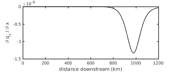
The calculation then, for a single \(t\) (which we implicitly set to be 1 second with out sediment transport calculation), the change in sediment transport capacity over space is maximized in the backwater region.

This vector is converted to the commensurate change in bed elevation over this single \(t\) by multiplying by \((1/(1-\lambda_p))\). Of course, we can consider many \(t\)s at once, and so the vector would again be multiplied by the timestep (\(\Delta t\)). We’ll consider this in the next post, where we add a time loop to the model, such that on ever timestep, the backwater, slope, sediment transport and change in bed elevation are each recalculated and updated so that we have a delta model which evolves in time!

The code for this part of the model is available here.

This material is based upon work supported by the National Science Foundation (NSF) Graduate Research Fellowship under Grant No. 145068 and NSF EAR-1427177. Any opinion, findings, and conclusions or recommendations expressed in this material are those of the author(s) and do not necessarily reflect the views of the National Science Foundation.