TeXlive install process, or developing an intelligent download timer: Part 2

In part one of this series, I presented the download predictions for a program installation. The ultimate goal here, is to develop a method for accurately predicting total download times from the beginning of the download process. To elaborate, as the download progresses, it should become increasingly easy to make an accurate prediction of the time remaining, because there is increasingly less and less to download, and you have increasingly more and more information about the download history.

Naturally, the first thing we want to do is see if the data actually follow any sort of trend. In theory, larger packages in the TexLive install should take longer, but the time/volume of each should be roughly the same, and should remain roughly constant (or really vary about some mean constantly) over time. The easiest way to determine this would be to simply plot the download speed over the duration of the download.

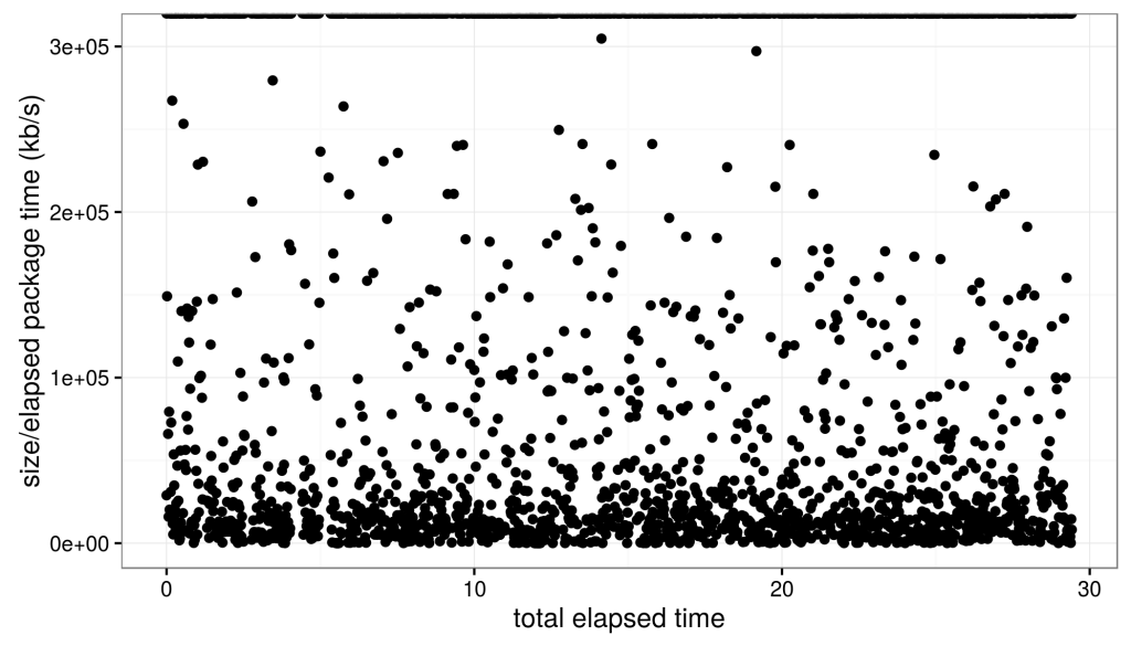
The speed varies significantly, but that’s okay. It, qualitatively, appears that the distribution of speeds randomly varies about a mean value. This is good for us, because it means that there is no trend in the speed over time, like we would see for example if the mean speed were changing over time.

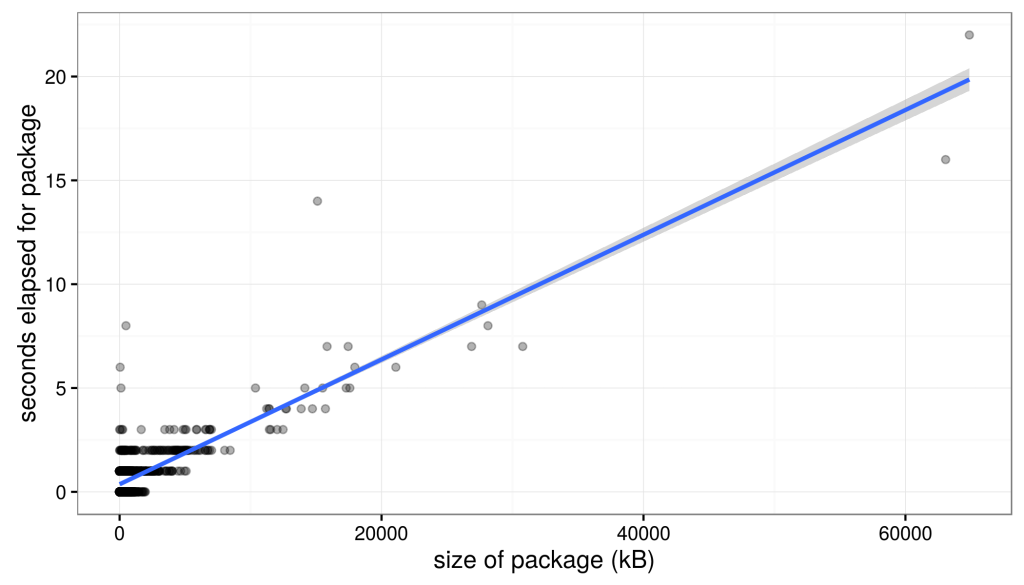
This means that we can build a model of download speeds to predict the total download time. If we simply fit a linear model to the data above (i.e., elapsed package time ~ size) we find that the data are reasonably well explained (r^2 = 0.60) by a line of slope = 3.003797e-4 and intercept = 3.661338e-1.

Then, we can use our linear model to evaluate, in essence, to predict the time it will take to download each package based on the size of each package and then sum them to produce a prediction for the total download time. Evaluation produces a predicted total download time of 29:26 mm:ss (plotted as dashed line below).

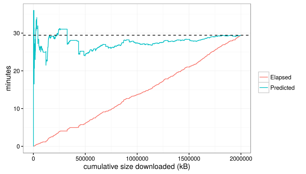
29:26 happens to be the exact time that our download took. That means that despite all the variations in download speeds, the mean over time was so constant that a simple linear model (a constant download speed) perfectly predicts the observed data; perhaps this is not surprising when you see the roughly constant-slope red line above.

Now, this model was based on perfect information at the end of the download, but in the next post, we’ll explore a common, simple, and popular prediction algorithm as a test of an a priori and ongoing prediction tool.